Background
This is a real take-home interview problem from Tesla Autopilot. I had an interview with them in May 2017. This is a very interesting and challenging problem.
Before I worked on this problem, the Tesla people didn’t even know whether this problem is NP-hard or not. The standard solution provided by Tesla people used an inferior approximation algorithm. However, as a rock star engineer, I discovered the optimal solution in hours and beat all the people in Tesla.
You can download the problem, data set and my solution in Google Drive.
Problem
The problem is to find the minimum time path for a Tesla car to drive from one charging station s to another charging station t in a Tesla charging station network. The car has a maximum range of 320km, so it needs to charge in intermediate stations. However, each station has a charging speed in km/hr, indicating how many more kilometers the car can drive per hour charging, before the car reach the 320km maximum range.
The input is the names of the starting station and the destination station. A header file is provided with a list of charging stations with their names, coordinates, and charging speeds.
The output is a single line in the following format: starting station name, first intermediate station name, charge time in hrs, second intermediate station name, charge time in hrs, …, …, destination station name.
Assumptions
(1) The car starts with a full range of 320km.
(2) Each charging station has a longitude-latitude coordinate. And the Earth is a sphere of radius 6356.752km.
(2) The car travels at a constant speed of 105km/hr along great circle routes between stations.
Example
For example the command ./solution Council_Bluffs_IA Cadillac_MI might return:
Council_Bluffs_IA, Worthington_MN, 1.18646, Albert_Lea_MN, 1.90293, Onalaska_WI,
0.69868, Mauston_WI, 1.34287, Sheboygan_WI, 1.69072, Cadillac_MI
Tesla’s Solution
The Tesla’s solution is simple: for each charging station a, subdivide it into m+1 vertices (a, 0), (a, 1), …, (a, m), where vertex (a, i) denotes the state that the car is at charging station a and it currently has i/m * 320 km range. Then, for every vertex (a, i), we add an edge to (a, i+1) with the time equal to the corresponding charging time. Also for any points (a, i) and (b, j), we add an edge between them if (i-j)/m * 320 km is greater or equal to the distance between charging station a and b, and the time of the edge is the corresponding travel time between these two stations. Then we can simply use any shortest path algorithm to find the shortest path between (s, m) and (t, 0) in the new graph and we can get a solution. Please note that this is an approximate algorithm, which means it just does not return the optimal solution. Since Tesla’s original problem description asked for optimal solution, Tesla’s own solution is technically wrong.Also, even though this algorithm is easy to reason about, it is actually much harder to implement comparing to my optimal solution. You will see how simple my code is in a moment.
A Polynomial Solution
The optimal solution is not as trivial as Tesla’s solution. We need to prove several lemmas first.
Lemma 1: If the distance between s and t is greater than the maximum range, the best solution always contain charging time greater than zero. Otherwise, the best solution is to go from s to t directly.
The proof is trivial.
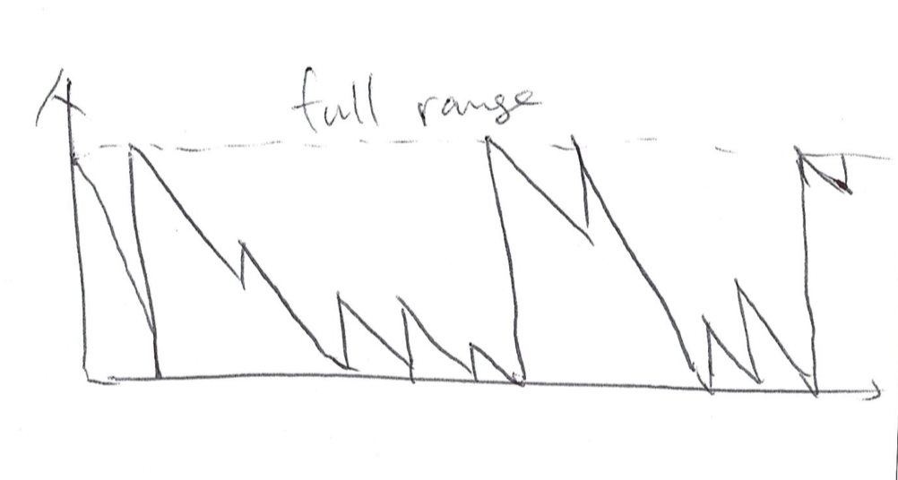
Lemma 2: In the optimal solution, we always reach the destination with the zero remaining range.
Proof: Assume that there is an optimal solution with non-zero remaining range r. Let a be the last station the car charged. And let r’ be the extra range we gain from the charging in station a. Now we construct a new solution where everything stays the same, except we charge min(r, r’) less in station a.
The new solution is a valid solution: before reaching a it is the same as the old solution; after reaching a and charging for the last time, in the new solution the car always has min(r, r’) less range than the old solution. Because we had range r remaining in the old solution, we will always have at least 0 range remaining in the new solution. Thus is is a feasible solution.
The new solution also takes less time than the original solution because min(r, r’) > 0 so we save some charging time. Thus it is a contradiction with the assumption that the old solution is an optimal solution. Then we proved Lemma 2 is true.

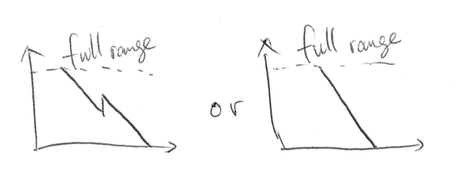
Lemma 3: There always exists an optimal solution where every intermediate station b has the following property: we always charge the car at b, and we either fully charge the car, or we charge just enough to reach the next station.
Proof: We will prove this lemma by contradiction. Assume that such optimal solution doesn’t exist. Then all solutions has some intermediate station doesn’t have the property Then let’s consider the solution with lowest number of stations in the output. If multiple such solutions exists, let’s consider the solution with lowest number of intermediate stations without the property.
Let’s consider an optimal solution with lowest number of stations in the output. We will prove that in such a solution, we either fully charge the car, or we charge just enough to reach the next station for every intermediate station.
For every three consecutive stations a, b, and c. We will consider all the cases: (1) We don’t charge at station b at all. (2) We charge less than enough to reach c. (3) We charge just enough to reach c. (4) We charge more than enough to reach c but do not fully charge. (5) We fully charge the car.
Case (3) and (5) are two permitted cases in Lemma 3. Case (2) is obviously impossible because we are not able to reach c if we didn’t charge enough in b. Now all we need is to prove that neither case (1) nor case (4) is impossible.
Case (1): Now assume that we don’t charge at station b at all. Then we can construct a new solution which is the same as the old solution except we skip station b. Since we didn’t charge at b in the old solution, the car has enough range to travel from a to b and c in the old solution. Therefore the car also has enough range to travel from a to c directly in the new solution. Therefore we found a solution with one less station and it takes at most as much time as the old solution. This is a contradiction with the fact that the old solution is an optimal solution with the lowest number of stations. Therefore we proved that case (1) is impossible for any intermediate station in such solutions.

Case (4): Assume that we charge at station b so that we have more than enough gas to reach c but not fully charge.
Because of Lemma 3 we know that c cannot be the destination, otherwise we will reach the destination with non-zero range, which is a contradiction because we just proved case (1) is impossible. Therefore we know c must be an intermediate station as well. There are 3 sub-cases:
Case (4.1): charging station in c is faster than b. Because we always charge and we charge more than enough in b. Therefore we can construct a new solution such that we charge a little bit less in b and a little bit more in c. Since charging station c is faster, the new solution is better, which is a contradiction.

Case (4.2): charging station in c is slower than b. Because we don’t fully charge at b and we always charge at c. We can construct a new solution such that we charge a little bit more in b and we charge a little bit less in c. Since c is slower, the new solution is better, which is a contradiction.

Case (4.3): charging station in c is as fast as b. There are 2sub-cases:
Case (4.3.1): we can skip charging station b in the old solution. Then construct a new solution by skipping b and charge more at c. We spend as much time in charging, spend at most as much time in traveling, but we have one less station in the new solution. It’s a contradiction with the fact that the old solution is an optimal solution with fewest number of stops.

Case (4.3.2): we cannot skip charging station b in the old solution. Then we charge just enough at b to reach c and we charge more at c. Then we constructed a new solution with the same travel time and the same charging time, and the total number of stations in the output is the same, and we have one less intermediate station without the property, which is a contradiction.

Algorithm
The first step of the algorithm is to handle the special case which we don’t need to charge at all. (Lemma 1)
With these Lemmas, we can construct a polynomial algorithm to find a optimal solution by search only paths where all intermediate station has the property in Lemma 3.
The algorithm has multiple passes of computations.
First, we compute the distance d_i,j between every pair of node.
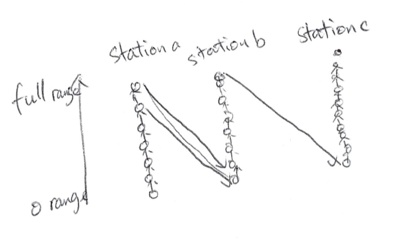
Second, we find the shortest-time path a0_i,j between every pair of stations such that we start with zero range, and reach the destination with zero range, and we never charge to the full range. By Lemma 3 we know that in this case we always charge just enough to reach the next station, thus we can use Floyd-Warshall algorithm to find all a1_i,j, using d_i,j and the corresponding charging time as edges.

Third, we find the shortest-time path a1_i,j between every pair of stations such that we start with full range, reach with zero range, and never reach zero range or full range in between. With Lemma 3 we know that there is only two possibilities: (1) the path has length 2 and the distance is the same as the range. (2) for all pats with length > 2, we know that in all intermediate station we can only charge enough to reach the next station, then the next station must has zero range. Then with the fact that we can only reach zero range in the destination we know that this path has length 3. Therefore we can compute all a1_i,j by brute force with O(n^3) complexity.

Fourth, we find the shortest-time path a2_i,j between every pair of stations such that we start with full range, reach with zero range, and never reach full range in between. They can be computed with all a1_i,k and a0_k,j pairs in O(n^3) time.

Fifth, we find the shortest path a3_i,j between every pair of stations such that we start with full range and reach with full range. This can be computed by using a second pass of Floyd-Warshall algorithm, with a2_i,j with charging time and d_i,j with charging time as edges.

Finally, because of Lemma 2, we can , consider all a2_s,t and all a3_s,k and a2_k,t to find the final solution.
Since every pass is O(n^3) time, the final algorithm is O(n^3).
My Program
This is my solution in C++. I used macros intensively. It’s generally not a good practice to use macros since it sometimes cause bugs without generating proper compilation errors. However in this particular problem I found macros very useful to beautify the code.
As you can see, even though the proof of this algorithm is very complicated, the actual program is surprisingly simple. The core of the program is only 10 line long, containing 4 passes of n^3 loops.An Even Better Algorithm
With the three lemmas we can find a solution even better than the one above.
This solution is a modification of Tesla’s solution. Instead of considering all possible range at every station, we only construct vertices for the full range, the empty range, the ranges such that it is just enough to reach another station, or the remaining range when we arrive the station from another station with full range. Then there are only O(n^2) vertices in this graph.
And then we add edges between stations only when the first vertex of the edge is full range or the second vertex of the edge is zero range. There are at most 2n^2 such edges. And we only add edges among vertices corresponding to a single station only if the second vertex of the edge is the next vertex with higher range comparing to the first vertex of the edge. There are at most 2n^2 such edges. Therefore the total number of edges is at O(n^2).
And then we can use Dijkstra algorithm to find the final solution.
The time to add edges is O(n^2 log n) because we need to sort the vertices corresponding to a single station. If we use Dijkstra algorithm with Fibonacci heap, the time complexity to find the shortest path is also O(n^2 log n). Therefore, the final time complexity of this algorithm is also O(n^2 log n).
Even though this algorithm is faster in complexity and easier to reason about, it is much harder to write the code down because I need to write the Dijkstra algorithm, an O(n log n) sorting algorithm, and a Fibonacci heap. Also in the 303 station network provided by Tesla, this algorithm is not necessarily faster. Therefore I didn’t implement this algorithm.
Aftermath of the Interview
#include "network.h"
#include

#define N 303
#define G 320.
#define V 105.
#define L 4
#define INF 67108864.
#define R 6356.752
#define SQ(x) ((x)*(x))
#define d2r(x) (x/180.*3.14159265358979323846264338327950288419716939937510)

#define LOOP(x,y) for(int x=0;x<y;++x)
#define LOOP(x) LOOP(x,N)
#define LOOP1 LOOP(i)
#define LOOP2 LOOP1 LOOP(j)
#define LOOP3 LOOP(k) LOOP2
#define RELAX(x,y,u,v) if(y<x){x=y;u=v;}

using namespace std;

string sn, tn;
int s,t;
double a[L][N][N], d[N][N], g[N];
int A[L][N][N];

bool input(int argc, char** argv) {
    if (argc != 3) return false;
    sn = argv[1];
    tn = argv[2];

    s = t = 0;
    while (s < network.size() && network[s].name != sn) ++s;
    while (t < network.size() && network[t].name != tn) ++t; if (s >= network.size() || t >= network.size()) return false;

    return true;
}

string output(int l, int i, int j) {
    if (i == j) return "";
    if (l == 0) {
        if (A[l][i][j] < 0)
            return " " + to_string(d[i][j]*g[i]/V) + " " + network[j].name;
        return output(0, i, A[l][i][j]) + output(0, A[l][i][j], j);
    }
    if (l == 1)
        return " " + network[A[l][i][j]].name + " "
        + to_string((d[i][A[l][i][j]]+d[A[l][i][j]][j]-G) * g[A[l][i][j]] / V)
        + " " + network[j].name;
    if (l == 2)
        return output(1, i, A[l][i][j]) + output(0, A[l][i][j], j);
    if (A[l][i][j] == -1)
        return output(2, i, j) + " " + to_string(g[j]/V);
    if (A[l][i][j] == -2)
        return " " + network[j].name + " " + to_string(d[i][j] * g[j] / V);
    return output(3, i, A[l][i][j]) + output(3, A[l][i][j], j);
}

int main(int argc, char** argv)
{
    if (!input(argc, argv)) {
        cout << "Error: requires initial and final supercharger names" << endl; return -1; } LOOP1 g[i] = V / network[i].rate; LOOP2 d[i][j] = R*2.*asin(sqrt(SQ(sin(d2r((network[i].lat-network[j].lat)/2.))) + cos(d2r(network[i].lat))*cos(d2r(network[j].lat)) * SQ(sin(d2r((network[i].lon-network[j].lon)/2.))))); LOOP2 if (d[i][j] > G) d[i][j] = INF;
    if (d[s][t] <= G) {
        cout << sn + " " + tn << endl; return 0; } LOOP(l,L) LOOP2 a[l][i][j] = INF; LOOP(l,L) LOOP2 A[l][i][j] = -1; LOOP2 a[0][i][j] = d[i][j] * (g[i]+1.); LOOP3 RELAX(a[0][i][j], a[0][i][k] + a[0][k][j], A[0][i][j], k); LOOP3 if (d[i][k] + d[k][j] >= G)
        RELAX(a[1][i][j], G + (d[i][k]+d[k][j]-G)*(g[k]+1.), A[1][i][j], k);

    LOOP3 RELAX(a[2][i][j], a[1][i][k] + a[0][k][j], A[2][i][j], k);

    LOOP2 a[3][i][j] = a[2][i][j] + g[j] * G;
    LOOP2 RELAX(a[3][i][j], d[i][j] * (1. + g[j]), A[3][i][j], -2);
    LOOP3 RELAX(a[3][i][j], a[3][i][k] + a[3][k][j], A[3][i][j], k);

    int m = INF, M = -1;
    LOOP1 RELAX(m, a[3][s][i] + a[2][i][t], M, i);
    if (M < 0)
        cout << "No path exists." << endl;
    else
        cout << sn + output(3, s, M) + output(2, M, t) << endl;

    return 0;
}
I didn’t get a job offer in the end. The coding challenge went well. The recruiter submitted my information to the hiring managers of two different teams. And then the asked me where I was from. I said “China”. Then the recruiter just stopped the interview process abruptly and denied my applications to both teams.
Lessons learned:
(1) Always reveal your ethnicity when applying for jobs. That’s why I have my photo in my homepage. The company is going to know your ethnicity sooner or later. It’s better to get discriminated before the interview starts so you don’t waste time. Also, I believe racism is fundamentally wrong ethically. If a company is practicing racism, you know they are evil and it would not be a good company to work for, regardless of your ethnicity. So reveal your ethnicity is a good way to efficiently avoid evil companies like Tesla.
(2) Never ever work on take-home interview problems. Your time is precious. For every hour you spend on your job application, you need to make sure someone at your level spend an hour on your application. This is very important to make sure they take your application seriously. 1-to-1 interviews are expensive for companies. Thus they give 1-to-1 interviews only after they review your background and experience, and think there is a good chance they will hire you. However, take-home problem is basically free for them. Their best strategy is to give take home problems to as many people as possible, and only start looking into your background and experience after you finish the problem. It means there is a good chance you will be rejected by something on your resume, even after you spend a long time working on their take-home interview problem.
Anyway, this problem is still my favorite interview problem of all time. There are three reasons.
(1) There are so much depth in this problem. There is an exponential brute force algorithm. There is an approximation algorithm. And we can find two polynomial algorithms if we spent time studying the properties of the optimal solutions. One of the polynomial algorithms is so simple that it just contains four 3D loops.
(2) This problem shows how much better I am comparing to the Tesla people.
(3) The background of this problem is so good. It vividly portrays the constant anxiety of the miserable Tesla owners. They need to worry about the battery life of their cars constantly since the range is so short and it’s so difficult to find a charging station. Even if they can find a charging station, after every hour of driving, they need to drive half an hour to the next Tesla supercharger and charge for half an hour. By comparison, with my very fuel inefficient Range Rover I can drive from Boston to Washington, D.C. without stopping at a gas station.
Sometimes I wonder why Tesla interview job candidates with a problem showing how bad their products are. But after I think about the fact that they couldn’t even solve this problem, I believe I know the answer.